My Grading Scheme

There is no universally-agreed-upon way to convert the overall score of a student to the final letter grade. Many institutions (including METU) leave this to the instructor’s full discretion, and many instructors choose to do this assignment in an heuristic course-by-course manner. I instead do this assignment in an algorithmic way, which is detailed in this website for full transparency.

Overview of different approaches

Let us assume that a student $S$ takes a class $C$: at the end of the semester, the grade $G$ of the student is expected to depend both on the student $S$ and the class $C$. Ideally, we would know the function $f$ such that $G=f(S,C)$, which completely takes into account both the student and the class.

Determining such a function $f$ would require us to have access to infinite information: the student may have infinitely many attributes that we should take into account (how much they study, how intelligent they are, if they lost a family member this semester, etc.), and the class may depend on infinitely many conditions (how good the instructor is, how hard the tests are, whether it is a morning class, etc.). It is impossible to find the “correct” $f$, even if it exists.

(a) The first practical approach that we can choose is to assume the following:

• The dependence on $S$ can be reduced to a single parameter: the score of the student.
• The dependence on $C$ can be ignored.

Under these assumptions, the letter grade can be assigned to a student solely based on their scores, independent of the semester of the course. Therefore, we simply create score brackets (such as 90-100, 85-90, etc.), and assign letter grades based on which bracket a student’s score falls into. This is colloquially called catalog grading.

(b) The second practical approach assumes the following:

• The dependence on $S$ can be reduced to a single parameter: the score of the student.
• There are sufficiently many students in the class.

In this approach, we argue that each student has some probability to obtain some score at the end of the semester; for instance, student 1 might have probability $1∕4$ to obtain a score greater than $70$ out of $100$. Therefore, we can assign a probability distribution to each student, telling us their likelihood to get some particular score (such as 72 or 49). Now, if we assume that (1) these probability distributions are sufficiently similar and (2) there are sufficiently many students in the class, the probability distribution for a hypothetical average student becomes a Gaussian distribution. This follows from the Central Limit Theorem.

The letter grades of individual students are now assigned based on how well they did compared to this hypothetical average student. For instance, if a student has the score $40$, and the probability for the hypothetical average student to get a score between $30$ and $100$ is $1∕100$, then the student is to be awarded the letter grade AA even though their score would be FF under the “catalog grading”. This “comparing with the gaussian” type of grading is colloquially called curve grading.

(c) There are several other approaches, which relax some of the assumptions in the other methods. For instance, one can extend the dependence on $S$ beyond the mere score of the student. This would entail including the observations of the student (such as class attendance) into the final letter grade. Despite having the potential to be somehow fairer, these methods are either non-algorithmic or non-practical for large classes, hence I do not prefer them.

My algorithm

There are some problems both with the catalog and traditional curve grading:

• They are ambiguous! In the catalog grading, there is no objective way to choose where to put the brackets: we could go with the standard brackets (90-100, 85-59, 80-84, etc.), but they are not dictated by a fair objective mechanism. The approach of the curve grading is better, but it also suffers from the same problem; for instance, if a student is in the top $15\%$ of the class, should s/he get AA, BA, or BB?
• They are unfair in the letter transitions! For instance, if we decide that a student gets AA above some particular score $X$, there may be 30 students in the class who get the the letter grade BA because their score is $X-1$, whereas 25 other students with the score $X+1$ get the letter grade AA: both catalog and traditional curve grading are insensitive to such problems!
• They cannot distinguish high effort from low effort! It is easier to get 5 more points if your grade is 20 out of 100, whereas this becomes extremely hard if your grade is 92. In other words, two students with the grades $20$ and $25$ can be considered to have put similar efforts, whereas another student pair with the grades $92$ and $97$ can not be considered in the same way. The traditional curve grading fits to a Gaussian curve, which is symmetric, therefore one should induce this asymmetry externally. In the catalog grading, there is no mechanism at all to supply such an asymmetry. In short, in both approaches, one relies on instructor’s judgement to ensure that the grading scheme distinguishes low and high efforts.

The first two problems can be solved if we cluster students into various groups: indeed, we expect students to obtain similar results if they turn in similar homeworks or make similar mistakes in the exams, so it is natural to observe clustering of students around some score points. If we identify such clusters and group them into 9 categories, we can assign letter grades in an unambiguous fair way!

There is a fast and reliable way to do just this: following Mathematica command splits the “scores” list into 9 categories, based on the clustering of the individual scores!

This, however, does not solve the third problem above as the clustering method does not distinguish different parts of the score spectrum. We can remedy this by stretching the high end of the scores and squeezing the low end –this can be achieved by the following code:

where $X\ge 100$ (with default value $100$) is a tunable parameter ensuring the asymmetry, with $X\to \infty$ restoring back the symmetry.

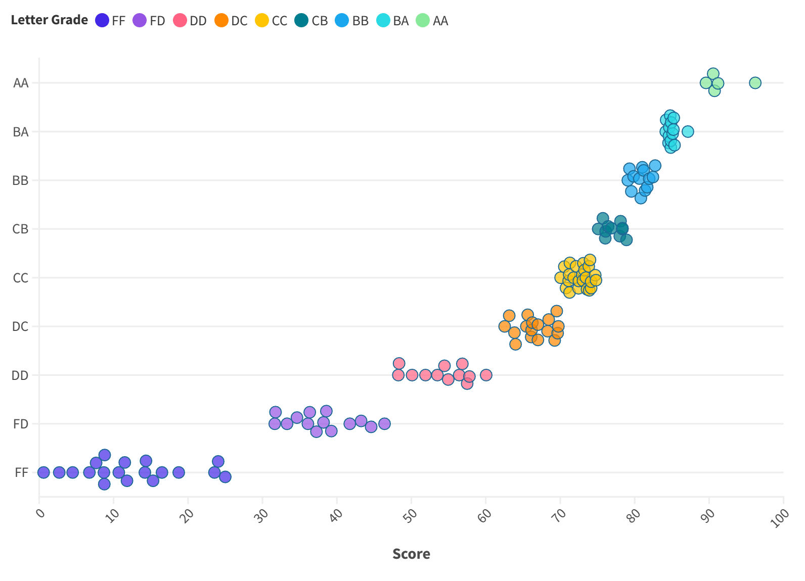
This ensures an algorithmic unambiguous grading scheme which tries to assign same letter grade to students with similar scores, and which distinguishes the effort to get more points between low and high end of the score spectrum. An actual example of how this approach led to letter grades can be seen in the following figure, which reflects the grades of my Phys209 class in 2023 Fall Semester.

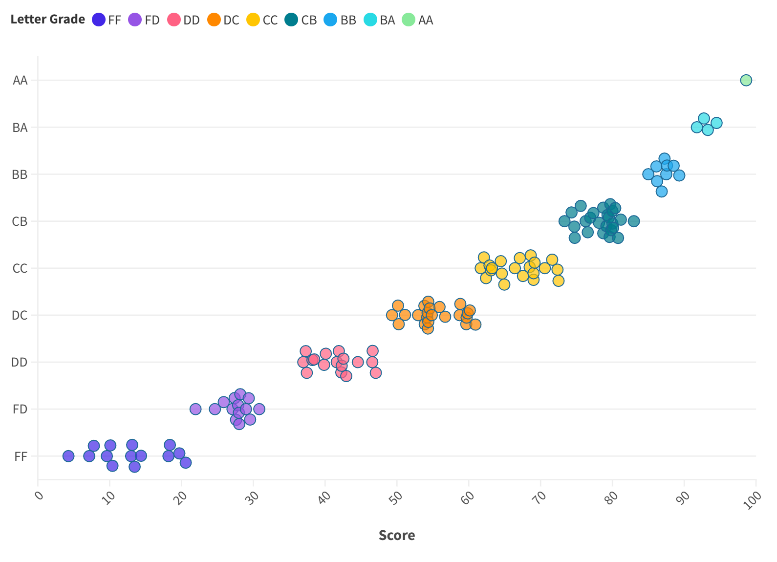
One problem with this approach is the effect of outlier students who receive rather high grades: the algorithm (by design) isolate them as the sole receipents of the letter grade AA, rendering other successful (but not outlier) students receiving lower letter grades. For instance, the algorithm yields the following distribution for my Phys209 class in 2024 Fall semester:

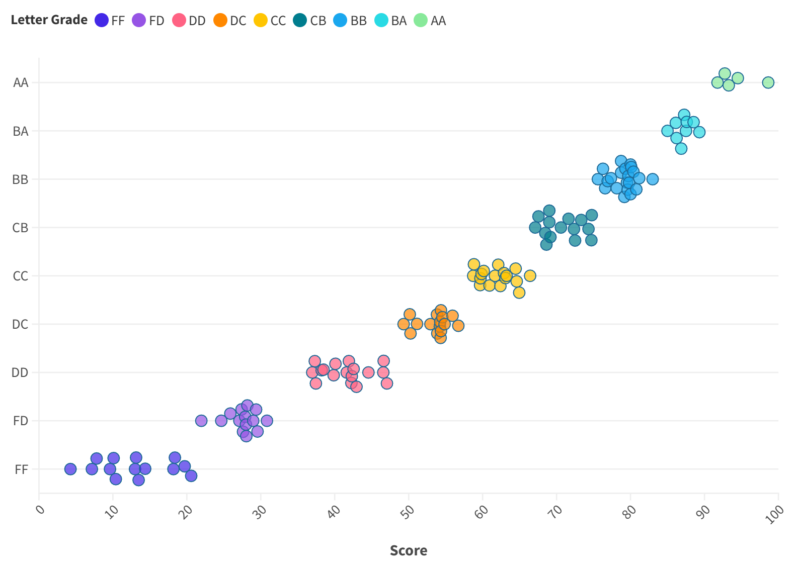
We can tweak the the parameter $X$ mentioned above to present this; we can also create more clusters and reward a few of the top clusters the grade AA. For example, for my Phys209 class in 2024 Fall semester, I created 10 clusters and awarded the top two groups the letter grade AA, leading the final distribution below.

Another solution is to explicitly specify a method for FindClusters command; for instance, for my Phys210 class in 2024 Spring semester, I chose KMeans method to ensure sufficiently many students get higher grades as can be seen in the comparison below.

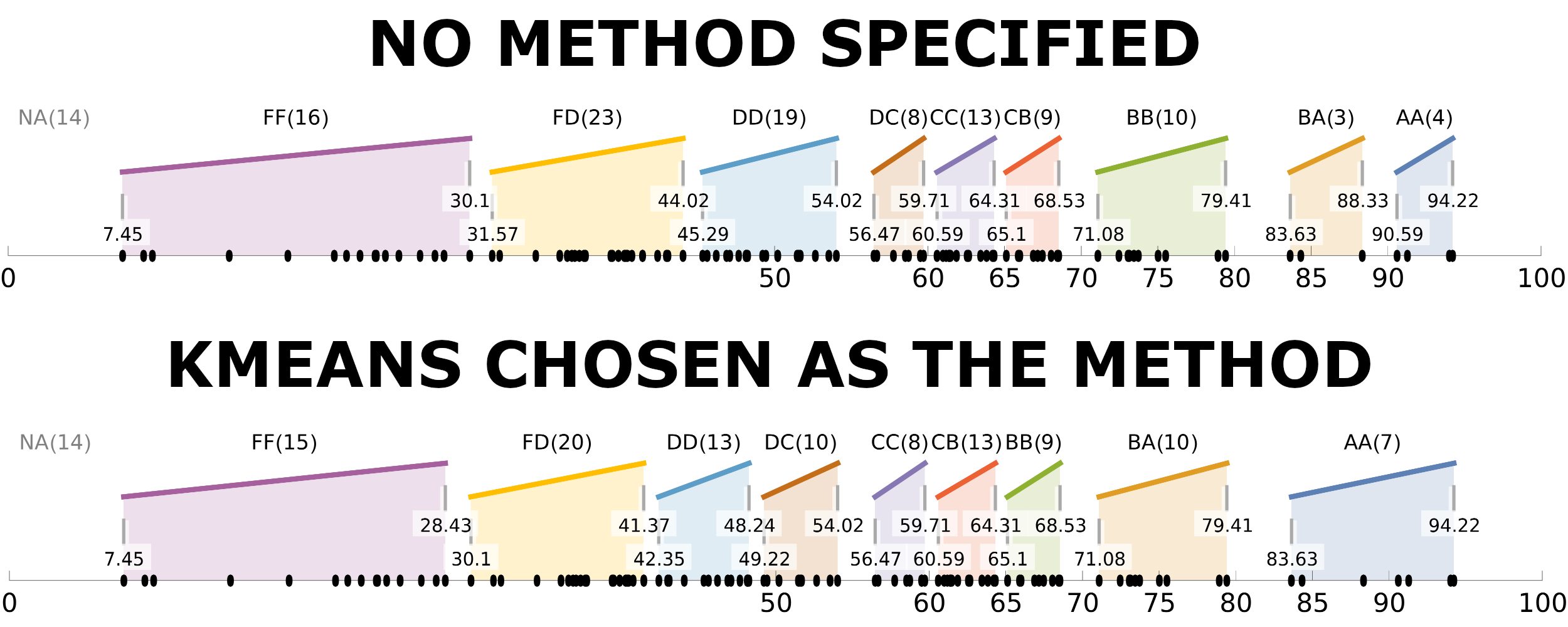
where I also took $X=110$ in this particular case.